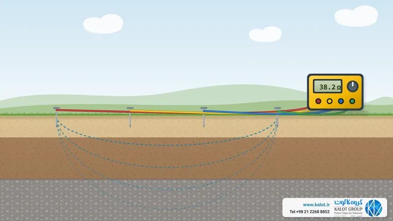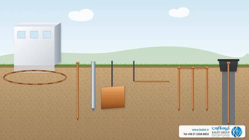
Earth resistance measurement means finding the resistance an earth termination (earth rod, plate, tape or earthing grid) presents to current flowing into the surrounding soil. The most common method is the three-point method, also called fall of potential (Fall-of-Potential): the earth tester sends an alternating current from the electrode under test to a remote auxiliary earth rod and measures the voltage with a second auxiliary earth rod driven at about 62% of that distance. Before an earthing system is designed, soil resistivity is also measured with the four-electrode Wenner or Schlumberger methods.
In this guide, we at KALOT Group explain all three methods step by step, with formulas, probe spacing, advantages, limitations and common errors, drawing on the reference standards and on application guides from respected makers of measuring instruments.
Two tests, two different questions
First of all, we need to be clear which quantity we are measuring:
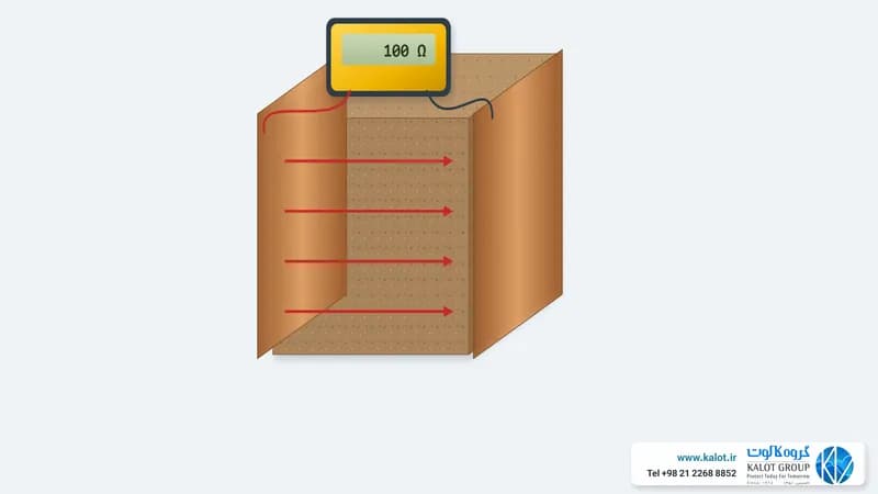
Earth termination resistance (earth resistance) | Soil resistivity (ρ) | |
|---|---|---|
Question | How many ohms is the installed earth termination? | How conductive is the soil on this site? |
Unit | Ohm (Ω) | Ohm-metre (Ω·m) |
When it is done | After installation, at handover and during periodic inspections | Before the earthing system is designed |
Common method | Three-point (fall of potential) and complementary methods | Wenner and Schlumberger (four-electrode) |
What the result is used for | Accepting or correcting the installed earth termination | Choosing the type, depth and number of electrodes, and the need for ground improvement material |
To learn what resistivity means and what affects it, see our guide to soil electrical resistivity. The value earth resistance should reach in each application is covered in our article on earth electrical resistance for different uses.
The three-point or fall-of-potential method (Fall-of-Potential)
How does this method work?
An earth tester has three terminals:
- E (electrode under test): connects to the earth termination of the building or installation.
- H or C (current electrode): the remote auxiliary earth rod that forms the return path for the test current.
- S or P (potential electrode): the intermediate auxiliary earth rod that senses the voltage.
The instrument drives a current I between E and H and reads the potential difference U between E and S. The termination resistance is then Rₑ = U / I.
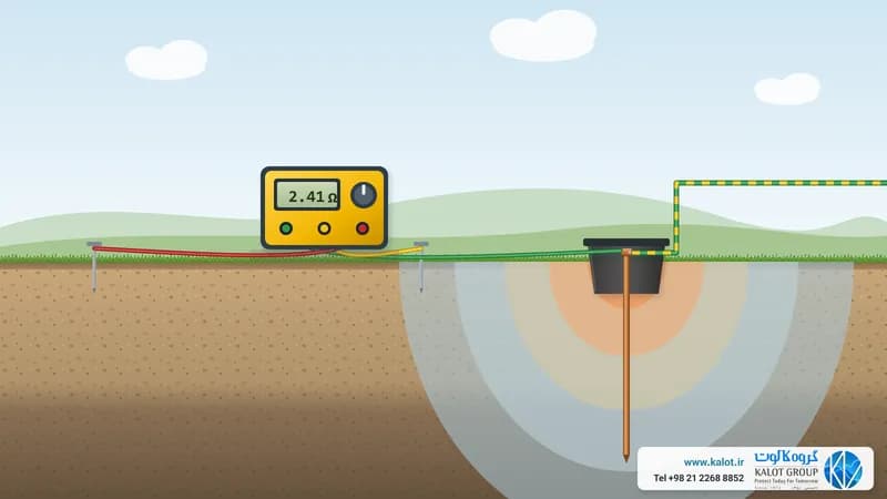
Every electrode has a zone of influence in the soil around it. The soil shells close to the electrode have little surface area, so most of the resistance is concentrated there. If we move S from E towards H, the reading first climbs quickly, then reaches a flat section (plateau), and rises sharply again near H. The correct resistance value is that flat section.
Why 62%?
Assuming uniform soil and hemispherical electrodes, the potential calculation shows that the point where the field of H is exactly cancelled lies at 61.8% of the distance from E to H. That is why we drive S at 0.62d, where d is the distance from E to H. The rule has three conditions: the soil must be roughly uniform, H must be far enough away that the zones of influence do not overlap, and all the test current must enter the soil through electrode E.
Before you start: safety notes
- Do not test during a thunderstorm or when lightning is possible.
- Before opening the link, use a clamp ammeter to check that no leakage or fault current is flowing in the earth conductor. If current is present, do not open the connection.
- Do not disconnect the earthing of a live installation without coordination and safety measures. During the test, connected equipment effectively has no protective earth.
- Use insulating gloves and footwear and suitable tools, and mark the cable routes for passers-by.
Steps of the three-point test
- Isolate the termination: open the test link on the main earth bar (MET) or the connection inside the earth inspection pit, so that only this termination is measured and parallel paths (network neutral, the earthing of other installations, pipes) stay out of the result.
- Set the distances: make the distance from E to H at least 5 times the largest dimension of the earthing system (for a grid, its diagonal). For a single earth rod, the distances in the table below are a common guide.
- Drive the auxiliary earth rods: drive H at distance d and S at 0.62d, with all three points in one straight line and in undisturbed soil.
- Lay the leads: unwind the leads fully from the reel, keep the current and potential leads apart, do not form loops, and do not run them parallel to buried cables, fences or rails.
- Check the auxiliary earth rods: read the resistance of the H and S probes on the instrument. If it exceeds the instrument's limit, drive the probe deeper, compact and moisten the surrounding soil, or add a second one in parallel about 2 m away.
- Main measurement: run the test with S at 0.62d and record the value. If the instrument has a noise indicator, change the test frequency.
- Check at 52% and 72%: move S once to 0.52d and once to 0.72d and measure again.
- Assess the result: if the three values differ by only a few per cent, their average is the termination resistance. If the difference is large (usually more than about 10%), S is still inside the zone of influence of E. Increase d and repeat the test.
- Test in another direction: to be sure, turn the test line by about 90 degrees and repeat. A large difference between the two directions points to buried metal, stray earth currents or non-uniform soil.
- Record and close the link: record the result, date, weather and soil moisture, distances, method and instrument, then close the test link again.
Common guide distances for a single earth rod:
Earth rod length | Distance of S from E | Distance of H from E |
|---|---|---|
2 m | about 15 m | about 25 m |
3 m | about 20 m | about 30 m |
6 m | about 25 m | about 40 m |
10 m | about 30 m | about 50 m |
For large grids and substations, the distance to H can reach several hundred metres.
The full method: plotting the curve
If time and space allow, move S from E to H in 10% steps and plot resistance against distance. A clear flat section means the test is valid. If the curve does not flatten, H is not far enough away.
Four-wire instead of three-wire connection
In a three-wire connection, the resistance of the E lead is added to the result. With a short lead the effect is negligible, but for very low resistances (a substation earthing grid, for example) a four-wire connection is used: a separate potential lead to the electrode removes the lead error.
Advantages and limitations of the three-point method
Advantages
- The reference method in the standards, accepted for handover tests and inspections.
- A direct result, with a way to check its accuracy (52/62/72% or plotting the curve).
- Fast and low in cost for a single electrode and for small to medium systems.
Limitations
- It needs open space and long cables, which is difficult in cities and on ground covered with concrete or asphalt.
- For large grids, distances reach hundreds of metres, and inductive coupling between the leads causes errors.
- The link has to be opened, which is not possible in some installations.
- Pipes, cables and buried metal distort the curve.
- In layered soil, the correct point may move away from 62%. Published research has shown that in large grids and non-uniform soil, reading directly at 61.8% can give a significant error, so plotting the curve or using the slope method is necessary.
- The result depends on the season and on soil moisture.
Complementary methods
- Slope method: for large grids whose electrical centre is unknown. From three readings at 20%, 40% and 60% of the distance, a ratio called μ is calculated, and the correct position of S is read from a standard table.
- Selective clamp method: a current clamp on the conductor of that electrode measures only its share without opening the link. It still needs auxiliary earth rods.
- Stakeless method (two-clamp): one clamp induces a voltage and the other measures the loop current. It is fast and needs no disconnection, but it works only when several parallel earth terminations form a return path. It does not work on a single electrode, and it measures the whole loop. It is useful for periodic monitoring, and an important result should be confirmed by the three-point method.
- Two-pole method: measures the electrode in series with an extensive metal system (metal pipework, for example). Use it only as a last resort and under strict conditions.
- High-current injection: for very large substations and grids, using several tens of amperes at a frequency close to the network frequency to reduce the effect of noise.
Measuring soil resistivity with four-electrode methods
In both methods, four test probes are driven in one line: the two outer ones, H and E, inject the current and the two inner ones, S and ES, measure the potential difference (ΔV). The instrument shows R = ΔV / I, and the formula for each arrangement gives the apparent resistivity of the soil. As the spacing grows, the current reaches deeper layers, which reveals how resistivity changes with depth.
The Wenner four-point method (Wenner)
In the Wenner method, the spacing between every two adjacent electrodes is d, and the resistivity is found from this relationship:
ρ = 2π d R
- ρ: soil resistivity (Ω·m)
- d: spacing between electrodes (m)
- R: resistance read by the instrument (Ω)
This relationship holds when the driving depth of the test probes is small compared with d. The common guidance from instrument makers and ASTM G57 is a driving depth of at most d/20. As a rule of thumb, each reading roughly represents the average soil down to a depth of about d.
Steps of the Wenner test
- Choose the location: a place that represents the site of the future earthing system, away from pipes, cables, fences and existing earthing grids.
- Set the line and spacings: mark a straight line and a centre point, and choose gradually increasing spacings, for example 1, 2, 3, 5, 7.5, 10, 15, 20, 30 and 40 m. The maximum d should be at least the largest dimension of the planned earthing system.
- Drive the test probes: drive all four at an equal spacing d, in one line and to a depth of less than d/20.
- Connect the leads: connect in the order H, S, ES, E, and keep the current and potential leads apart.
- Measure: enter d in the instrument or calculate ρ from the formula. Check the resistance of the auxiliary probes and record R.
- Next spacing: move all four probes to the next spacing and repeat the test.
- Perpendicular direction: repeat the whole test along a line perpendicular to the first.
- Plot on site: plot ρ against d on a logarithmic graph. The curve should be smooth. A sudden jump means you should check the connection or the probe.
- Interpretation: a flat curve means roughly uniform soil. A rising curve means a more resistive lower layer (rock or dry gravel). A falling curve means a more conductive lower layer (wet clay or groundwater).
Advantages of the Wenner method: simple geometry and a direct formula; the strongest voltage signal among the common arrangements, and so better resistance to noise; well suited to detecting horizontal soil layering; the most widely used method in the electrical industry.
Limitations of the Wenner method: all four probes must move at each step, so the test takes time; large spacings need very long cables; surface non-uniformity near the potential electrodes has a greater effect on the result.
The Schlumberger method (Schlumberger)
In the Schlumberger method (its name is spelled differently in some sources), the two potential electrodes S and ES sit at the centre of the arrangement with a small, fixed spacing A, and only the current electrodes H and E move gradually outward. If d is the distance from each current electrode to the neighbouring potential electrode:
ρs = π d (d + A) R / A
- ρs: apparent soil resistivity (Ω·m)
- d: distance from each current electrode to the neighbouring potential electrode (m)
- A: spacing between the two potential electrodes (m)
- R: resistance read by the instrument (Ω)
If you measure the distance from the centre of the arrangement to each current electrode (L) instead of d, the same relationship is written as ρs = π (L² − A²/4) R / A, and both give the same result. If d equals A, the arrangement is the Wenner one and the relationship becomes ρ = 2πAR.
Steps of the Schlumberger test
- Centre and potential electrodes: mark the centre of the line and drive S and ES on either side of it with spacing A (1 m, for example).
- Current electrodes: drive H and E symmetrically at distance d from the potential electrodes, in the same line. The driving depth of all electrodes should be small compared with the spacings (about one-twentieth).
- Connect the leads: as in the Wenner method, in the order H, S, ES, E.
- Measure: enter A and d in the instrument or calculate ρs from the formula. Record R, the current and the resistance of the auxiliary probes.
- Move the current electrodes out: move only H and E further away in increasing steps and repeat the test.
- Change A if needed: when the voltage reading becomes too small, increase A. At the same current electrode position, take one reading with the old A and one with the new A, so the two parts of the curve join up.
- Perpendicular direction and curve: repeat the test in the perpendicular direction and plot ρs against the distance from the centre to the current electrode on a logarithmic graph.
Advantages of the Schlumberger method: faster and less laborious, since only two electrodes move in most steps; better suited to investigating deeper layers with a smaller spread; and because the potential electrodes stay fixed, surface non-uniformity around them has less effect on the curve.
Limitations of the Schlumberger method: the voltage between the potential electrodes is small and falls quickly as the distance grows, so a more sensitive instrument is needed; A sometimes has to be changed and the two parts of the curve joined; the calculation and interpretation are a little more complex.
Comparing the Wenner and Schlumberger methods
Feature | Wenner | Schlumberger |
|---|---|---|
Spacing | All spacings equal (d) | Small, fixed potential spacing A; variable current spacing |
Formula | ρ = 2πdR | ρs = πd(d + A)R / A |
Electrodes moved at each step | 4 | 2 (A only occasionally) |
Signal level | High | Lower; a more sensitive instrument is needed |
Sensitivity to surface non-uniformity | Higher | Lower |
Speed of work on site | Slower | Faster |
Suitable for | General applications and high-noise environments | Investigating deeper layers and large sites |
The measuring instrument: which features matter?
- Alternating, not direct, current: direct current polarises the contact surface between electrode and soil and puts an error in the result. Standard earth testers inject alternating current (usually a square wave) at a frequency well away from 50 Hz and its harmonics. Common frequencies lie between about 40 and 130 Hz.
- Noise rejection and frequency selection: in industrial environments and near substations, being able to change the frequency or have it selected automatically is important.
- Checking the auxiliary earth rods: the instrument should measure the resistance of the H and S probes and warn if it is too high.
- Three-wire and four-wire modes and automatic resistivity calculation for Wenner and Schlumberger.
- Compliance with IEC 61557-5, the standard for earth resistance measuring equipment.
Common measurement errors
- Not opening the test link: the result includes parallel paths and reads lower than the true value.
- H too close: the zones of influence overlap and the curve does not flatten.
- Buried metal near the test line: a pipe, cable, fence or existing earthing grid.
- Leads running parallel and close together: inductive coupling between the current and potential leads, especially over long distances.
- Driving the test probes too deep in a resistivity test: the simple formula is no longer valid.
- Testing in only one direction: lateral non-uniformity in the soil goes unseen.
- Not plotting the curve on site: wrong readings are discovered too late.
- Ignoring the season: a test right after rainfall shows a lower resistance than dry summer conditions.
Season, inspection intervals and recording results
Earth resistance changes with soil moisture, temperature and freezing, and the surface layers change the most. Design should be based on the worst seasonal conditions, and deeper electrodes usually give a more stable value.
For lightning protection systems, IEC 62305-3 recommends these inspection intervals (national regulations take precedence):
Protection level | Visual inspection | Full inspection (with testing) | Sensitive systems |
|---|---|---|---|
I and II | Every 1 year | Every 2 years | Full inspection every 1 year |
III and IV | Every 2 years | Every 4 years | Full inspection every 1 year |
At every test, record the value of each test link (open), the total value (closed), the method and instrument, the distances, the date and the soil condition (dry, wet, frozen), and compare with earlier results. A noticeable increase points to corrosion, a loosened connection or drying soil.
How do measurement results help with design and equipment selection?
- Soil model: Wenner or Schlumberger data are converted into a uniform or two-layer model. For the design of substation earthing grids, IEEE 80 takes at least a two-layer model as its basis.
- Deep or wide? If the conductive layer is deep, copper-bonded earth rods with a steel core and deep electrodes are more effective. If the surface layer is more conductive, choose tape and horizontal conductors and a wider grid.
- High-resistivity soil: on rocky, dry ground, ground improvement materials help reduce and stabilise termination resistance. To estimate the quantity needed, see the GIM calculator.
- Allowing for periodic testing: the earth termination should be testable from day one. An earth inspection pit and an earth bar make it easy to reach the test link.
To calculate the resistance of simple electrodes before installation, see the article How is earth termination resistance calculated?
Our specialists at KALOT Group are ready to work with you. Send us your soil resistivity results, the site dimensions and the type of use, and we will help you choose the right electrode, conductor, connections and ground improvement material. For advice, contact us.
Reference standards
IEEE Std 81 (2025 edition) · IEEE Std 80 · BS 7430 · IEC 62305-3 · IEC 61557-5 · IEC 60364-6 · EN 50522 · ASTM G57